Our Previous Samples

ECO6214: Module 7: Exam II

Score for this quiz: 150 out of 150
Submitted May 1 at 2:13am
This attempt took 55 minutes.

 
Question 1                                            10 / 10 pts
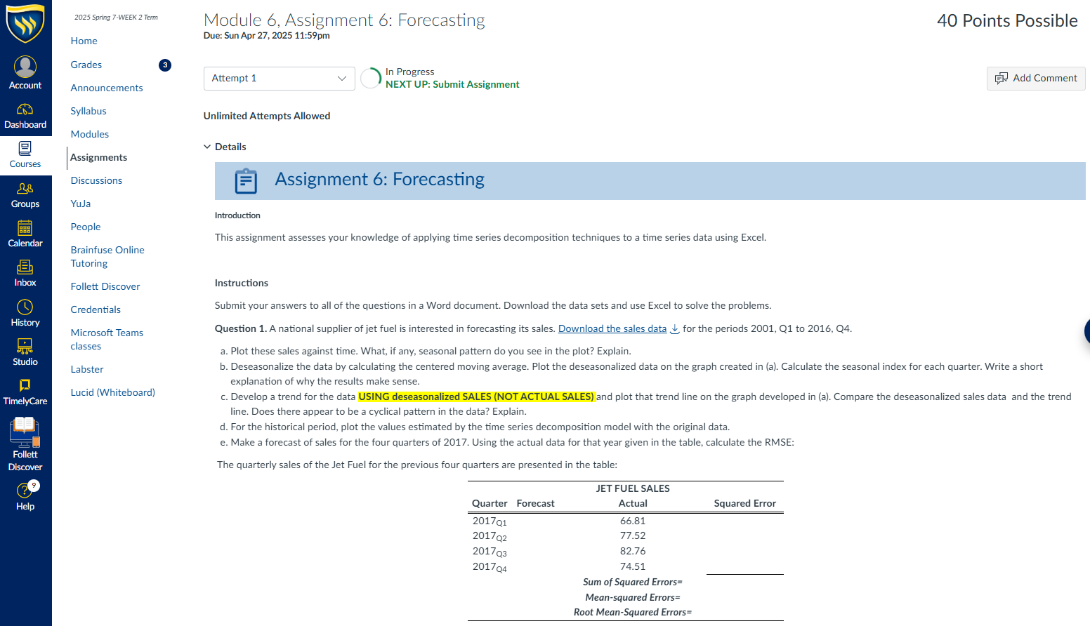
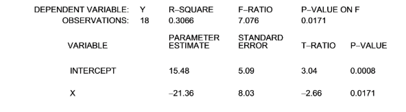
The linear regression equation, Y = a + bX, was estimated. The following computer printout was obtained:

The parameter estimate of  a indicates

•   when X is zero, Y is 15.48
•   when Y is zero, X is 8.03
•  when Y is zero, X is -21.36
•  when X is zero, Y is 5.09.

 
Question 2                                            10 / 10 pts
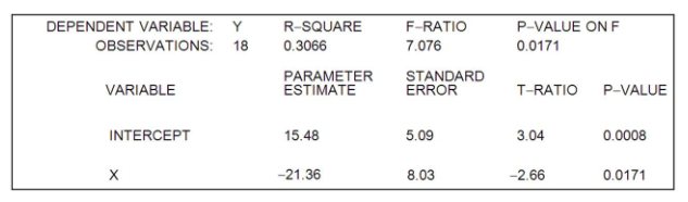
The linear regression equation, C = a + bQ+cQ, was estimated. The following computer printout was obtained:

The value of R2 indicates that _______ of the total variation in C is explained by the regression equation. 

•   7.679%
•   76.79%
•   7679%
•   0.7679%

 
Question 3                                            10 / 10 pts
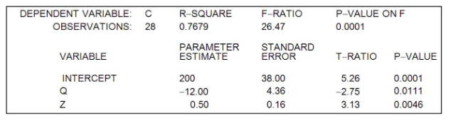
The manufacturer of Beanie Baby dolls used quarterly price data for 2005I-2013IV (t = 1, ..., 36) and the regression equation:

to forecast doll prices in the year 2014. Pt is the quarterly price of dolls, and,  and  are dummy variables for quarters I, II, and III, respectively.

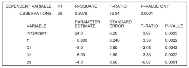
What is the estimated intercept of the trend line in the 3th quarter?

•  22.8
•  25
• 18
• 16
• 20

 
Question 4                                            10 / 10 pts
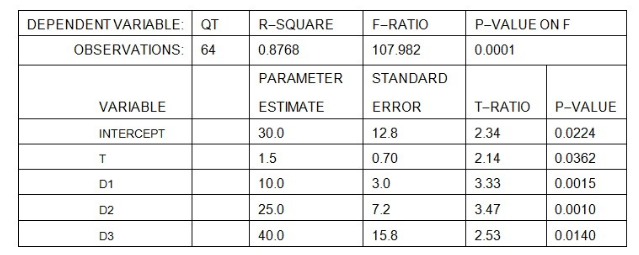
A forecaster used the regression equation

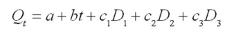
and quarterly sales data for 1996I-2013IV (t = 1, ..., 64) for an appliance manufacturer to obtain the results shown below. Q is quarterly sales, and ,  and  are dummy variables for quarters I, II, and III.

Using a 5 percent significance level, these estimation results indicate that

•   sales in the fourth quarter are significantly greater than sales in any other quarter.
•   sales in the third quarter are significantly greater than sales in any other quarter.
•   sales in the second quarter are significantly greater than sales in any other quarter.
•   sales in the first quarter are significantly greater than sales in any other quarter.

 
Question  5                                            10 / 10 pts
When the correlation coefficient is negative, it means:

• when X goes down, Y does too.  
• Y will not be a good predictor of X.  
• X will not be a good predictor of Y.  
• when X goes down, Y tends to go up.   
• there is a weak relationship.

 
Question  6                                           10 / 10 pts
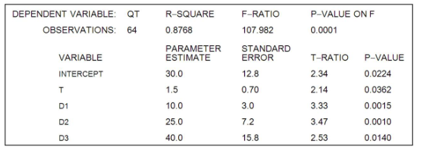
Thirty data points on Y and X are employed to estimate the parameters in the linear relation Y = a + bX. The computer output from the regression analysis is:

The parameter estimate of a (intercept) indicates

•   when Y is zero, X is -3.25.  
• when Y is zero, X is 93.54.  
• when X is zero, Y is -3.25.  
• when X is zero, Y is 93.54.

Question  7                                          10 / 10 pts
The linear regression equation, Y = a + bX, was estimated.  The following computer printout was

obtained:

Given the above information, which of the following statements is correct at the 1% level of significance?

•   â (intercept) is statistically significant, but  (slope) is not
•   Both â(intercept) and  (slope) are statistically significant.
•   (slope) is statistically significant, but â (intercept) is not.
•   Neither â intercept) nor  (slope) is statistically significant.

 
Question  8                                          10 / 10 pts
The linear regression equation, Y = a + bX, was estimated.  The following computer printout was

obtained:

Given the above information, if X equals 20, what is the predicted value of Y?

•   -411.72  
• 186.42  
• -186.42  
• 165.69

 
Question  9                                          10 / 10 pts
A forecaster used the regression equation
Qt = a + bt +c1D1 +c2D2 + c3D3

and quarterly sales data for 1996I-2013IV (t = 1, ..., 64) for an appliance manufacturer to obtain the results shown below. Q is quarterly sales, and D1,D2 and D3 are dummy variables for quarters I, II, and III. 

What is the estimated intercept of the trend line in the second quarter?

•   49
•   65
•   26.6
•   25
•   55

 
Question  10                                          10 / 10 pts
A forecaster used the regression equation
Qt = a + bt +c1D1 +c2D2 + c3D3

and quarterly sales data for 1996I-2013IV (t = 1, ..., 64) for an appliance manufacturer to obtain the results shown below. Q is quarterly sales, and D1,D2 and D3 are dummy variables for quarters I, II, and III. 

At the 5 percent level of significance, is there a statistically significant trend in sales?

•   Yes, because 2.14 >0.05.
•   No, because 1.5 > 0.05.
•   Yes, because 0.700 > 0.05.
•   Yes, because 0.0362 < 0.05

 
Question  11                                          10 / 10 pts
A firm is experiencing theft problems at its warehouse. A consultant to the firm believes that the dollar loss from theft each week (T) depends on the number of security guards (G) and on the unemployment rate in the county where the warehouse is located (U measured as a percent). In order to test this hypothesis, the consultant estimated the regression equation T = a + bG + cU and obtained the following results: 

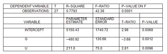
Based on the above information, hiring one more guard per week will decrease the losses due to theft at the warehouse by _________ per week.

•  $5,150
•   $211
•   $480.92
•   $130

 
Question  12                                          10 / 10 pts
For the equation Y = a + bX, the objective of regression analysis is to

• estimate the variables Y and X.
• estimate the parameters a and b.

 
Question  13                                         10 / 10 pts
In a linear regression equation of the form Y = a + bX, the intercept parameter b shows

• the increase in the value of X when Y increases by 1 unit.
• the increase in the value of Y when X increases by 1 unit.

 
Question  14                                         10 / 10 pts
If an analyst believes that more than one explanatory variable explains the variation in the dependent variable, what model should be used?

• a multiple regression model  
• binary model  
• a simple linear regression model  
• quadratic model

 
Question  15                                          10 / 10 pts
Income is used to predict savings. For the regression equation Y = 1,000 + .10X, which of the following is true?

• Y is income, X is savings, and income is the independent variable.  
• Y is income, X is savings, and savings is the independent variable.  
• Y is savings, X is income, and income is the independent variable.  
• Y is savings, X is income, and savings is the independent variable.

Instructions

Submit your answers to all of the questions in a Word document. Download the data sets and use Excel to solve the problems.

Question 1. A national supplier of jet fuel is interested in forecasting its sales. Download the sales data  for the periods 2001, Q1 to 2016, Q4.

• Plot these sales against time. What, if any, seasonal pattern do you see in the plot? Explain.
• Deseasonalize the data by calculating the centered moving average. Plot the deseasonalized data on the graph created in (a). Calculate the seasonal index for each quarter. Write a short explanation of why the results make sense.
• Develop a trend for the data USING deseasonalized SALES (NOT ACTUAL SALES) and plot that trend line on the graph developed in (a). Compare the deseasonalized sales data  and the trend line. Does there appear to be a cyclical pattern in the data? Explain.
• For the historical period, plot the values estimated by the time series decomposition model with the original data.
• Make a forecast of sales for the four quarters of 2017. Using the actual data for that year given in the table, calculate the RMSE:

 The quarterly sales of the Jet Fuel for the previous four quarters are presented in the table:

Introduction

This discussion assignment gives you the opportunity to research the four components of the time series decomposition technique. You will consult academic sources and explain the four components without using technical jargon.

Instructions

In your own words, write a description of each of the four components of the classic time series decomposition technique. Do your best to avoid using mathematical relationships and technical jargon so that your explanations can be understood by small business owners. Please cite at least two academic sources.

This discussion can be conducted as a roleplay activity. Each student will assume the role of an audience member who is a small business owner and will ask a question about forecasting in plain language. Each of you, in your role as an expert, will answer the question. Your classmates will answer your question, and you will answer the questions posted by your classmates.

Introduction

This assignment assesses your understanding of and ability to apply multiple regression models to a series of business data using the Excel Analysis ToolPak.

Instructions

Submit your answers to all of the questions in a Word document. Download the data sets and use Excel to solve the problems.

Question 1. Download the data and develop a multiple-regression model for auto sales as a function of population and household income for 10 metropolitan areas.

1. Estimate values for b₀, b₁, and b₂ for this model:
   AS = b₀ + b₁ (INC) + b₂ (POP)
2. Are the signs you find for the coefficients consistent with your expectations? Explain.
3. What percentage of variation in AS is explained by this model?
4. What point estimate of AS would you make for a city where INC=23,175 and POP=128.7?

Question 2. The quarterly sales of the TRK-50 mountain bike for the previous four years by a bicycle shop in Switzerland are presented in the table:

1. Plot the sales against time.
2. Use the data to estimate the monthly trend in sales using a linear trend model of the form:
   Q_t = a + bt. Does your statistical analysis indicate a trend? If so, is it an upward or downward trend and how great is it? Is it a statistically significant trend at 5 percent level of significance?
3. Now adjust your statistical model to account for seasonal variation in sales. Estimate this model of sales:
   Q_t = a + bt + cD₂ + dD₃ + eD₄
   where D₂, D₃, D₄ are the appropriately defined dummy variables for quarters 2, 3, and 4.
   Do the data indicate a statistically signifi¬cant seasonal pattern at 5 percent level of significance? If so, what is the seasonal pattern of sales?
4. Comparing your estimates of the trend in sales in parts b and c, which estimate is likely to be more accurate? Why?
5. Using the estimated forecast equation from part c, forecast sales for Quarters 1 and 4 of 2014 and Quarters 2 and 3 of 2015.

Submission

• Submit your answers in a Word document.
• Submit the Excel files to show your calculations.
• Include the relevant graphs of actual and forecast values of the series. Please do not forget to title your graph.

Submit your calculations and answers in a 1–3-page document and spreadsheet to the Dropbox by Day 7 of the week.

Introduction

This discussion provides you with an opportunity to discuss the use of dummy variables for capturing seasonality in the data.

Instructions

Respond to these questions:

• Explain what dummy variables are and how they can be used to account for seasonality.
• Please cite at least one academic article (APA or MLA format). 
• Select a product or service of your choice and explain how you would use dummy variables to measure seasonality in the sales of that product or service.
• Explain the expected sign of each dummy variable.

Directions

• Make your initial post by Day 4 of this week and comment on at least two of your classmates’ posts by Day 7.
• Post your response to the discussion and then read your classmates’ posts. Post TWO responses to at least TWO of your classmates' posts. Initial post should be no less than 150 words and no more than 450 words.
• Discussions need to be professional. Please make proper use of capitalization and punctuation and make sure that there are no misspellings, incomplete sentences, or other grammatical errors.
• The basic criterion for a discussion post to be considered effective is that your message is original and intelligible. You must communicate concisely and clearly.

Introduction

This assignment assesses your understanding of the simple linear regression model and provides you with an opportunity to apply this method to forecast data.

Instructions

Submit your answers to all questions in a Word document. Download the data sets and use Excel to solve the problems.

Question 1. Carolina Wood Products, Inc., a major manufacturer of household furniture, is interested in predicting expenditures on furniture (FURN) for the entire United States. You are going to help the company with this prediction. Download the data by quarter for 2007 through 2016.

1. Estimate the bivariate linear trend model for the data where TIME=1 for 2007, Q1 through TIME=40 for 2016, Q4.

   FURN = a + b(TIME)

2. Evaluate this model in one paragraph, with particular emphasis on its usefulness in forecasting.
3. Prepare a time-trend forecast of furniture and household equipment expenditures for 2017 based on the model in (b).

   Period	Time	Trend Forecast
   2017 Q1	41
   2017 Q2	42
   2017 Q3	43
   2017 Q4	44

Question 2. Alexander Enterprises manufactures plastic parts for the automotive industry. Download data on its sales (in thousands of dollars) for 2012, Q1 through 2016, Q4. You are to forecast sales for 2017, Q1 through 2017, Q4.

1. Begin by preparing a time series plot of the data set. Does it appear from this plot that a linear trend model will be appropriate? Explain. (Attach your graph to your answer.)
2. Use a bivariate linear regression trend model to estimate this trend equation:
   SALES = a + b(TIME)
   Is the sign of b what you would expect? Is b significantly different from zero? What is the coefficient of determination for this model? Explain your answers.
3. Based on this model, make a trend forecast of sales (SALESFT) for the four quarters of 2017.
4. The actual sales (SALESA) for the four quarters are provided in the table.

   2017, Q1	4447.1
   2017, Q2	4501.6
   2017, Q3	4543.2
   2017, Q4	4603.1

Calculate RMSE for this forecast model in the historical period (2012, Q1–2016, Q4) as well as for the forecast horizon (2017, Q1–2017, Q4). Which of these measures accuracy and which measures fit?

Submission

• Submit your answers in a Word document.
• Submit the Excel files to show your calculations.
• Include the relevant graphs of actual and forecast values of the series. Please do not forget to title your graph.

Submit your calculations and answers in a 1–3-page document and spreadsheet to the Dropbox by Day 7 of this week.

Introduction

This discussion allows you to discuss and apply the linear trend model for forecasting total house sales in the United States.

Instructions

Download the data on annual historical total houses sold (THS) in the U.S. and its regions. Select a region you are interested in and get the last 20 years of data.

To prepare for the discussion, undertake the analysis on the given points:

• By using a bivariate regression trend line model, forecast total houses sold for the next five years.
• Prepare a time series plot of these data (years are on the x axis, THS is on the y axis) that shows both actual and forecast THS for the next five years.

Post the results of your statistical analysis and the graph with your response to the following:

• Do you think the model looks as though it will provide reasonably accurate forecasts for a five-year horizon? Explain your answer.

HINTS:

• The data set in the discussion includes multiple spreadsheets. You will need to use the data on the first spreadsheet (Sol Ann). Choose a region from this spreadsheet and extract 20 years of house sales data (1996-2016). Next, use a linear trend model to forecast the next five years.
• I have also created a video demonstrating the use of a linear trend model with Texas population data. Please watch the video, and if you have any questions, please let me know.

Linear Trend Model with Texas Population Data.

• Refer to the given video if you do not know how to estimate data with a trend line in Excel.

Corman, L. (2010, September 28). Trend lines and regression analysis in excel. [Video file] [14 min 43 sec]. Retrieved from https://www.youtube.com/watch?v=6rOlGbLeQxI

Directions

• Make your initial post by Day 4 of this week and comment on at least two of your classmates' posts by Day 7.
• Post your response to the discussion and then read your classmates’ posts. Post TWO responses to at least TWO of your classmates' posts. Initial post should be no less than 150 words and no more than 450 words.
• Discussions need to be professional. Please make proper use of capitalization and punctuation and make sure that there are no misspellings, incomplete sentences, or other grammatical errors.
• The basic criterion for a discussion post to be considered effective is that your message is original and intelligible. You must communicate concisely and clearly.

Expert Answer

Introduction

This assignment assesses your understanding of the forecasting methods you have learned this week and gives you an opportunity to compare and evaluate the results of different forecasting methods.

Instructions

Submit your answers to all questions in a Word document. Download the data sets and use Excel to solve the problems.

Question: Download the data on thermostat sales.

• Calculate both the three-month and the five-month averages for these data.
• Plot the data to examine the possible existence of trend and seasonality.
• Prepare the following two (2) separate forecasting models to examine the thermostat’s sales data using monthly data:

• • An exponential smoothing model (α=0.38, smoothing constant for the level)
  • Holt’s model (α=0.04, smoothing constant for the level; β=0.07, smoothing constant for the trend)

        d. Examine the accuracy of the forecast given by each model ( four models: MA 3, MA 5, Simple Exponential smoothing and  Holt's Method) by calculating the root mean square error (RMSE) for each during the historical period.

        e. Which model does minimize the RMSE? Carefully explain which characteristics of the original data caused one of these models to minimize the RMSE.

         f. Using Holt's method forecast 12 months of thermostat sales for 2017.

Hints:

Part e: In this task, you will calculate four Root Mean Square Errors (RMSE), one for each model (MA3, MA5, Simple Exponential Model, and Exponential Model with Trend-Holt’s Method). The MA3 and MA5 models are used to forecast stationary data (without trend). The Simple Exponential Model is used to forecast stationary data (without trend), while the Exponential Model with Trend-Holt’s Method is used to forecast non-stationary data (with trend).

Visualizing the data will help you detect any data patterns such as trend, seasonality, or stationary data with random errors. This will assist you in answering part e of the task.

Part f: In the lecture notes, the embedded video on Holt's Method did not explain how to forecast future data using Holt's Method. To forecast with Holt's Method, use the following algebraic form:

Ht+m = Ft+m * Tt

Here, Ht+m represents Holt’s forecast value for period t+m. Please watch virtual lab 3 recordings to learn how to complete this part.

Virtual Lab 3.

Assignment 3's dataset is larger than the previous assignments, and thus, you can limit the amount of data that you report in the Word document by following the instructions below:

Part A: Report a table that includes the last five periods of forecast (MA3 and MA5), including January 2017. Alternatively, you can include a plot of actual and forecast data.

Part B: Include a plot of actual data along with an explanation.

Part C: Report a table that includes the last five periods of forecast (Simple Exponential Smoothing and Holt's), including January 2017. Alternatively, you can include a plot of actual and forecast data. Please refer to the videos I posted to make a forecast with Simple Exponential Smoothing and Holt's.

Part D: Report the RMSE's of all four models.

Part E: Provide an explanation.

Part F: Include a table that shows a 12-month forecast with Holt's Method.

Submission

• Submit your answers in a Word document.
• Submit the Excel files to show your calculations.
• Include the relevant graphs of actual and forecast values of the series. Please do not forget to title your graph.

Submit your calculations and answers in a 1–3-page document and spreadsheet to the Dropbox by Day 7 of this week.

Module 3, Midterm Exam

Attempt 1   Score for this quiz: 90 out of 120
Submitted Apr 6 at 7:16pm
This attempt took 32 minutes.

 
Question 1                                     10 / 10 pts
Under what circumstances may it make sense NOT to prepare a business forecast?
  

• No data is readily available.  
• There is no consensus among informed individuals.  
• The industry to forecast is undergoing dramatic change.  
• The future will be no different from the past.  
• The forecast horizon is 40 years.

 
Question 2                        5 / 5 pts
Which subjective forecasting method depends upon the anonymous opinion of a panel of individuals to generate sales forecasts?  

• None of the above.
• Sales Force Composites.
• Jury of Executive Opinion.
• Customer Surveys.
• Delphi Method.

 
Question 3                              5 / 5 pts
Which of the following is NOT considered a subjective forecasting method?

•   Consumer surveys.
•   Juries of executive opinion.
•   Sales force composites.
•   Naive methods.
•   Delphi methods.

 
Question 4             5 / 5 pts
Suppose you are attempting to forecast a variable that is independent over time such as stock rates of return. A potential candidate-forecasting model is
  

• The Delphi Method.  
• None of the above.  
• The Jury of Executive Opinion.  
• Last period’s actual rate of return.  
• Last period’s actual rate of return plus some proportion of the most recently observed rate of change in the series.

 
Question 5                               5 / 5 pts
Of the following model selection criteria, which is often the MOST important in determining the appropriate forecast method?

•  Technical background of the forecast user.
•  When is the forecast needed?
•  What is the forecast horizon?
•  Patterns the data have exhibited in the past.
•  How much money is in the forecast budget?

 
Question 6                 5 / 5 pts
Which time-series component is said to fluctuate around the long-term trend and is fairly irregular in appearance?

•   Cyclical.
•   Irregular.
•   None of the above.
•   Seasonal.
•   Trend.

 
Question 7                                      10 / 10 pts
For which data frequency is seasonality not a problem?

•   Annual.
•   Daily.
•   Monthly.
•   Weekly.
•   Quarterly.

 
Question 8                                            5 / 5 pts
When a time series contains no trend, it is said to be

•   nonseasonal.
•   seasonal.
•   nonstationary.
•   stationary.
•   filtered.

 
Question 9             10 / 10 pts
A large sample of X-Y data values are analyzed and reveal a correlation coefficient of-.88. Which statement is correct?

•   The correlation is weak because r is less than -1.
•   There is no relation. 
•   A weak negative relationship exists.
•   A fairly strong negative linear relationship exists. *
•    If r had been +.88, the correlation would have been much stronger.

 
Question 10                      10 / 10 pts
Which method uses an arithmetic mean to forecast the next period?

•   Exponential smoothing.
•   Adaptive filtering.
•   Moving averages.
•   None of the above
•   Naive.

 
Question 11                            10 / 10 pts

If a three-month moving-average model is used, what is the forecast for period 4?

•   107.1.
•   108.3.
•   110.2.
•    106.6.
•   104.4.

 
Question 12                      10 / 10 pts

If a smoothing constant of .3 is used, what is the exponentially smoothed forecast for period 3?

•   103.0.
•   106.6.
•   115.0.
•   104.4.
•   112.6.

 
Question 13                                     10 / 10 pts

The ACF for The Gap sales is shown above. There is clear evidence in the ACF that

•   Gap sales have fallen in the last 12 periods.
•   there is a strong trend in the data.
•   the data is too strongly correlated to identify trend.
•   the data is stationary.
•   there is no seasonality in the data.

 
Question 14                        10 / 10 pts
If the correlation between body weight and annual income were high and positive, we could conclude that

•   high incomes cause people to gain weight.
•   high income people tend to be heavier than low income people, on average.
•   low incomes cause people to eat less food.
•   high incomes cause people to eat more food.
•   high income people tend to spend a greater proportion of their income on food than low income people, on average.

 
Question 15                                  10 / 10 pts
In the Holt's two-parameter smoothing model, the trend smoothing parameter Gamma

•   should be close to one when α is one.
•   should be close to one when the data has a relatively smooth trend.
•   should be close to one when α is close to one.
•   should be close to zero when the data has a relatively smooth trend.

Introduction

This assignment will test your knowledge of basic statistical concepts, the components of time series data, and using a correlogram for model selection.

Instructions

Submit your answers to all questions in a Word document. Download the data sets and use Excel to solve the problems.

Question 1. Thirty graduate students were asked how many credit hours they were taking in the current quarter. Download the available dataDownload Download the available data

1. Calculate the mean, median, standard deviation, variance, and range for this sample using Excel. Write a sentence explaining what each measure means.
2. What is the standard error of the mean based on the data?
3. What would be the best point estimate for the population credit hours? (“Population” refers to all graduate students’ credit hours in the universe.)
4. What is the 95% confidence interval for the means of credit hours? What is the 90% confidence interval?

Question 2. An investment manager has been working on a report for forecasting Apple stock price. Your job is to help him to determine whether there is a trend and/or seasonality in Apple stock prices. Download the dataDownload Download the data

1. Prepare a time series plot of these data.
2. Include a trend line using the Excel Analysis ToolPak. On the basis of your analysis, do you think there is a significant trend in Apple stock prices? Explain.

Watch the following video to learn how to add a trendline:

Watch the video: How to Add a TrendlineLinks to an external site. 

1. Is there seasonality? Explain.
2. What forecasting method might be appropriate for Apple stock prices according to the guidelines provided in your Table 2.1 (Chapter 2, page 58) of your textbook?

Question 3. The given figure is the correlogram for the total number of houses in the U.S. (quarterly data).

On the basis of the correlogram, do you think there is a significant trend? Explain.

Submission

• Submit your answers in a Word document.
• Submit the Excel files to show your calculations.
• Include the relevant graphs of actual and forecast values of the series. Please do not forget to title your graph.

Submit your calculations and answers in a 1–3-page document and spreadsheet to the Dropbox by Day 7 of this week.